5 Summary Statistics
Please load the following packages and data frame for this chapter:
library(tidyverse)
library(magrittr)
url <- "http://www.phonetik.uni-muenchen.de/~jmh/lehre/Rdf"
vdata <- read.table(file.path(url, "vdata.txt"))
When you want to get an overview of some data, it is helpful to compute so called summary statistics (sometimes called descriptive statistics). Among others, these are the arithmetic mean, median, variance, standard deviation, minimum, maximum, etc. Here we aim to show you how these values can be computed without using functions from the tidyverse. Since R is a statistics software, functions to compute summary statistics are always available. The following code snippet presents the most important functions from base R for descriptive statistics, applied to the F1 values in vdata:
## [1] 407.3## [1] 366## [1] 21255## [1] 145.8## [1] 0## [1] 1114## [1] 0 1114## 25%
## 300## 75%
## 509.8## [1] 209.85.1 Mean & Median
The arithmetic mean is calculated by summing \(n\) numbers and then dividing this sum by \(n\). Here is a very simple example:
## [1] 15## [1] 5## [1] 3## [1] 3The median on the other hand is the middle number in a sorted sequence of numbers. Let’s reuse the above example (in which the numbers are already in ascending order):
## [1] 1 2 3 4 5## [1] 3For an even number of numbers the median is the mean of the two middle values, e.g.:
## [1] 3.5## [1] 3.5The median is more robust against outliers than the mean. Outliers are data points that are more extreme then the majority of data points in a data set. Here is another simple example:
## [1] 1 2 3 4 5 100## [1] 19.17## [1] 3.5The number 100 is obviously an outlier in the vector called nums. Because of that, the mean is now much higher than previously, while the median has changed only slightly.
5.2 Variance & Standard Deviation
Variance and standard deviation are related measures for the dispersion of values around their mean. More precisely, the variance is the sum of the squared deviations of the values from their mean, divided by the number of values minus 1, while the standard deviation is the square root of the variance. The following example demonstrates how to compute the variance and standard deviation manually.
## [1] 12.4## [1] 0.16 40.96 134.56 88.36 21.16## [1] 5## [1] 285.2## [1] 71.3## [1] 71.3To compute the standard deviation from that (which is used far more often in statistics than the variance) we only need to extract the square root of the variance:
## [1] 8.444## [1] 8.4445.3 Quantiles
A quantile divides data points in such a way that a given part of the data points is below the quantile. Quantile is a hypernym: depending on how many chunks you divide your data points into, you can also use the terms percentile (100 chunks) or quartile (4 chunks). The median is another quantile because 50% of the data are below the median. In R, the function quantile() computes quantiles. The function takes as arguments the data points (i.e. a numeric vector) and then the proportion of data points that should be below the value to be computed. Important quantiles are the first and third quartile, i.e. the thresholds below which a quarter or three quarters of all data points lie.
## 25%
## 300## 75%
## 509.8## [1] 209.8The difference between the first and third quartile is called interquartile range and can be computed with the function IQR().
5.4 Example of a Boxplot
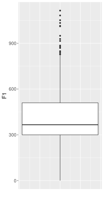
A boxplot contains many of the descriptive information that we have learned about so far:
- Median: the horizontal line within the box is the median.
- Box: the box contains the middle 50% of the data points. The lower end of the box is the first quartile (Q1), the upper end is the third quartile (Q3). The box is as big as the interquartile range.
- Whiskers: the vertical lines stretching upwards/downwards from Q1 and Q3 to the highest/lowest data point that lies within
1.5 * IQR. The calculation of the whiskers as1.5 * IQRis valid for boxplots created withggplot2, but some other programs use a different calculation. - Points: outliers, i.e. all data points that are not contained in the box or whiskers.
Here you see a boxplot for F1 from the data frame vdata:

Later in this course, you’ll learn how to create this boxplot yourself.